Higher-order critical points: definitions and curiosities
\newcommand{\abs}[1]{\left|{#1}\right|} \newcommand{\argmax}[1]{\underset{#1}{\operatorname{argmax}}} \newcommand{\argmin}[1]{\underset{#1}{\operatorname{argmin}}} \newcommand{\bareta}{{\overline{\eta}}} \newcommand{\barf}{{\overline{f}}} \newcommand{\barg}{{\overline{g}}} \newcommand{\barM}{\overline{\mathcal{M}}} \newcommand{\barnabla}{\overline{\nabla}} \newcommand{\barRcurv}{\bar{\mathcal{R}}} \newcommand{\barRmop}{\bar{R}_\mathrm{m}} \newcommand{\barRmoptensor}{\mathbf{{\bar{R}_\mathrm{m}}}} \newcommand{\barx}{{\overline{x}}} \newcommand{\barX}{{\overline{X}}} \newcommand{\barxi}{{\overline{\xi}}} \newcommand{\bary}{{\overline{y}}} \newcommand{\barY}{{\overline{Y}}} \newcommand{\bfeta}{{\bm{\eta}}} \newcommand{\bfF}{\mathbf{F}} \newcommand{\bfOmega}{\boldsymbol{\Omega}} \newcommand{\bfR}{\mathbf{R}} \newcommand{\bftheta}{{\bm{\theta}}} \newcommand{\bfX}{{\mathbf{X}}} \newcommand{\bfxi}{{\bm{\xi}}} \newcommand{\bfY}{{\mathbf{Y}}} \newcommand{\calA}{\mathcal{A}} \newcommand{\calB}{\mathcal{B}} \newcommand{\calP}{\mathcal{P}} \newcommand{\calC}{\mathcal{C}} \newcommand{\calE}{\mathcal{E}} \newcommand{\calF}{\mathcal{F}} \newcommand{\calG}{\mathcal{G}} \newcommand{\calH}{\mathcal{H}} \newcommand{\calJ}{\mathcal{J}} \newcommand{\calK}{\mathcal{K}} \newcommand{\calL}{\mathcal{L}} \newcommand{\ones}{\textbf{1}} \newcommand{\calM}{\mathcal{M}} \newcommand{\calN}{\mathcal{N}} \newcommand{\calO}{\mathcal{O}} \newcommand{\calS}{\mathcal{S}} \newcommand{\calT}{\mathcal{T}} \newcommand{\calU}{\mathcal{U}} \newcommand{\calV}{\mathcal{V}} \newcommand{\calW}{\mathcal{W}} \newcommand{\calX}{\mathcal{X}} \newcommand{\Cm}{{\mathbb{C}^m}} \newcommand{\CN}{{\mathbb{C}^{\,N}}} \newcommand{\Cn}{\mathbb{C}^n} \newcommand{\CNN}{{\mathbb{C}^{\ N\times N}}} \newcommand{\Cnn}{\mathbb{C}^{n\times n}} \newcommand{\CnotR}{{\mathbb{C}\ \backslash\mathbb{R}}} \newcommand{\col}{\operatorname{col}} \newcommand{\im}{\operatorname{im}} \newcommand{\complex}{{\mathbb{C}}} \newcommand{\Cov}{\mathbf{C}} \newcommand{\Covm}{C} \newcommand{\Ric}{\mathrm{Ric}} \newcommand{\Rmcurv}{\mathrm{Rm}} \newcommand{\D}{\mathrm{D}} \newcommand{\dblquote}[1]{``#1''} \newcommand{\dd}[1]{\frac{\mathrm{d}}{\mathrm{d}#1}} \newcommand{\ddiag}{\mathrm{ddiag}} \newcommand{\ddp}[2]{\frac{\partial #1}{\partial #2}} \newcommand{\Ddq}{\frac{\D}{\dq}} \newcommand{\dds}{\frac{\mathrm{d}}{\mathrm{d}s}} \newcommand{\Ddt}{\frac{\D}{\dt}} \newcommand{\ddt}{\frac{\mathrm{d}}{\mathrm{d}t}} \newcommand{\Ddttwo}{\frac{\D^2}{\dt^2}} \newcommand{\defeq}{\triangleq} \newcommand{\Dexp}{\D\!\exp} \newcommand{\error}{\mathrm{error}} \newcommand{\diag}{\mathrm{diag}} \newcommand{\Diag}{\mathrm{Diag}} \newcommand{\Vol}{\mathrm{Vol}} \newcommand{\polylog}{\mathrm{polylog}} \newcommand{\poly}{\mathrm{poly}} \newcommand{\dist}{\mathrm{dist}} \newcommand{\Dlog}{\D\!\log} \newcommand{\dmu}{\mathrm{d}\mu} \newcommand{\dphi}{\mathrm{d}\phi} \newcommand{\dq}{\mathrm{d}q} \newcommand{\ds}{\mathrm{d}s} \newcommand{\dt}{\mathrm{d}t} \newcommand{\dtau}{\mathrm{d}\tau} \newcommand{\dtheta}{\mathrm{d}\theta} \newcommand{\du}{\mathrm{d}u} \newcommand{\dx}{\mathrm{d}x} \newcommand{\Ebad}{E_\textrm{bad}} \newcommand{\Egood}{E_\textrm{good}} \newcommand{\eig}{{\mathrm{eig}}} \newcommand{\ellth}{$\ell$th } \newcommand{\embdist}{\mathrm{embdist}} \newcommand{\ER}{{Erd\H{o}s-R\'enyi }} \newcommand{\Exp}{\mathrm{Exp}} \newcommand{\expect}{\mathbb{E}} \newcommand{\expectt}[1]{\mathbb{E}\left\{{#1}\right\}} \newcommand{\expp}[1]{{\exp\!\big({#1}\big)}} \newcommand{\feq}{{f_\mathrm{eq}}} \newcommand{\FIM}{\mathbf{F}} \newcommand{\FIMm}{F} \newcommand{\floor}[1]{\lfloor #1 \rfloor} \newcommand{\flow}{f_{\mathrm{low}}} \newcommand{\FM}{\mathfrak{F}(\M)} \newcommand{\frobnorm}[2][F]{\left\|{#2}\right\|_\mathrm{#1}} \newcommand{\frobnormbig}[1]{\big\|{#1}\big\|_\mathrm{F}} \newcommand{\frobnormsmall}[1]{\|{#1}\|_\mathrm{F}} \newcommand{\GLr}{{\mathbb{R}^{r\times r}_*}} \newcommand{\Gr}{\mathrm{Gr}} \newcommand{\grad}{\mathrm{grad}} \newcommand{\Hess}{\mathrm{Hess}} \newcommand{\HH}{\mathrm{H}} \newcommand{\Id}{\operatorname{Id}} % need to be distinguishable from identity matrix \newcommand{\II}{I\!I} \newcommand{\inj}{\mathrm{inj}} \newcommand{\inner}[2]{\left\langle{#1},{#2}\right\rangle} \newcommand{\innerbig}[2]{\big\langle{#1},{#2}\big\rangle} \newcommand{\innersmall}[2]{\langle{#1},{#2}\rangle} \newcommand{\ith}{$i$th } \newcommand{\jth}{$j$th } \newcommand{\Klow}{{K_{\mathrm{low}}}} \newcommand{\Kmax}{K_{\mathrm{max}}} \newcommand{\kth}{$k$th } \newcommand{\Kup}{{K_{\mathrm{up}}}} \newcommand{\Klo}{{K_{\mathrm{lo}}}} \newcommand{\lambdamax}{\lambda_\mathrm{max}} \newcommand{\lambdamin}{\lambda_\mathrm{min}} \newcommand{\langevin}{\mathrm{Lang}} \newcommand{\langout}{\mathrm{LangUni}} \newcommand{\length}{\operatorname{length}} \newcommand{\Log}{\mathrm{Log}} \newcommand{\longg}{{\mathrm{long}}} \newcommand{\M}{\mathcal{M}} \newcommand{\mle}{{\mathrm{MLE}}} \newcommand{\mlez}{{\mathrm{MLE0}}} \newcommand{\MSE}{\mathrm{MSE}} \newcommand{\N}{\mathrm{N}} \newcommand{\norm}[1]{\left\|{#1}\right\|} \newcommand{\nulll}{\operatorname{null}} \newcommand{\hull}{\mathrm{hull}} \newcommand{\Od}{{\mathrm{O}(d)}} \newcommand{\On}{{\mathrm{O}(n)}} \newcommand{\One}{\mathds{1}} \newcommand{\Op}{{\mathrm{O}(p)}} \newcommand{\opnormsmall}[1]{\|{#1}\|_\mathrm{op}} \newcommand{\p}{\mathcal{P}} \newcommand{\pa}[1]{\left(#1\right)} \newcommand{\paa}[1]{\left\{#1\right\}} \newcommand{\pac}[1]{\left[#1\right]} \newcommand{\pdd}[1]{\frac{\partial}{\partial #1}} \newcommand{\polar}{\mathrm{polar}} \newcommand{\Precon}{\mathrm{Precon}} \newcommand{\proj}{\mathrm{proj}} \newcommand{\Proj}{\mathrm{Proj}} \newcommand{\ProjH}{\mathrm{Proj}^h} \newcommand{\PSD}{\mathrm{PSD}} \newcommand{\ProjV}{\mathrm{Proj}^v} \newcommand{\qf}{\mathrm{qf}} \newcommand{\rank}{\operatorname{rank}} \newcommand{\Rball}{R_{\mathrm{ball}}} \newcommand{\Rcurv}{\mathcal{R}} \newcommand{\Rd}{{\mathbb{R}^{d}}} \newcommand{\Rdd}{{\mathbb{R}^{d\times d}}} \newcommand{\Rdp}{{\mathbb{R}^{d\times p}}} \newcommand{\reals}{{\mathbb{R}}} \newcommand{\Retr}{\mathrm{R}} \newcommand{\Rk}{{\mathbb{R}^{k}}} \newcommand{\Rm}{{\mathbb{R}^m}} \newcommand{\Rmle}{{\hat\bfR_\mle}} \newcommand{\Rmm}{{\mathbb{R}^{m\times m}}} \newcommand{\Rmn}{{\mathbb{R}^{m\times n}}} \newcommand{\Rmnr}{{\mathbb{R}_r^{m\times n}}} \newcommand{\Rmop}{R_\mathrm{m}} \newcommand{\Rmoptensor}{\mathbf{{R_\mathrm{m}}}} \newcommand{\Rmr}{\mathbb{R}^{m\times r}} \newcommand{\RMSE}{\mathrm{RMSE}} \newcommand{\Rn}{{\mathbb{R}^n}} \newcommand{\Rnk}{\mathbb{R}^{n\times k}} \newcommand{\Rnm}{\mathbb{R}^{n\times m}} \newcommand{\Rnn}{{\mathbb{R}^{n\times n}}} \newcommand{\RNN}{{\mathbb{R}^{N\times N}}} \newcommand{\Rnp}{{\mathbb{R}^{n\times p}}} \newcommand{\Rnr}{\mathbb{R}^{n\times r}} \newcommand{\Rp}{{\mathbb{R}^{p}}} \newcommand{\Rpp}{\mathbb{R}^{p\times p}} \newcommand{\Rrn}{{\mathbb{R}^{r\times n}}} \newcommand{\Rrr}{\mathbb{R}^{r\times r}} \newcommand{\Rtt}{{\mathbb{R}^{3\times 3}}} \newcommand{\sbd}[1]{\sbdop\!\left({#1}\right)} \newcommand{\sbdop}{\operatorname{symblockdiag}} \newcommand{\sbdsmall}[1]{\sbdop({#1})} \newcommand{\Sd}{\mathbb{S}^{d}} \newcommand{\Sdd}{{\mathbb{S}^{d\times d}}} \newcommand{\short}{{\mathrm{short}}} \newcommand{\sigmamax}{\sigma_{\operatorname{max}}} \newcommand{\sigmamin}{\sigma_{\operatorname{min}}} \newcommand{\sign}{\mathrm{sign}} \newcommand{\ske}{\operatorname{skew}} \newcommand{\Skew}{\operatorname{Skew}} \newcommand{\skeww}[1]{\operatorname{skew}\!\left( #1 \right)} \newcommand{\Sm}{\mathbb{S}^{m-1}} \newcommand{\smallfrobnorm}[1]{\|{#1}\|_\mathrm{F}} \newcommand{\Smdmd}{{\mathbb{S}^{md\times md}}} \newcommand{\Smm}{{\mathbb{S}^{m\times m}}} \newcommand{\Sn}{\mathbb{S}^{n-1}} \newcommand{\Snn}{{\mathbb{S}^{n\times n}}} \newcommand{\So}{{\mathbb{S}^{1}}} \newcommand{\SOd}{\operatorname{SO}(d)} \newcommand{\SOdm}{\operatorname{SO}(d)^m} \newcommand{\son}{{\mathfrak{so}(n)}} \newcommand{\SOn}{{\mathrm{SO}(n)}} \newcommand{\sot}{{\mathfrak{so}(3)}} \newcommand{\SOt}{{\mathrm{SO}(3)}} \newcommand{\sotwo}{{\mathfrak{so}(2)}} \newcommand{\SOtwo}{{\mathrm{SO}(2)}} \newcommand{\Sp}{{\mathbb{S}^{2}}} \newcommand{\spann}{\mathrm{span}} \newcommand{\gspan}{\mathrm{gspan}} \newcommand{\Spp}{{\mathbb{S}^{p\times p}}} \newcommand{\sqfrobnorm}[2][F]{\frobnorm[#1]{#2}^2} \newcommand{\sqfrobnormbig}[1]{\frobnormbig{#1}^2} \newcommand{\sqfrobnormsmall}[1]{\frobnormsmall{#1}^2} \newcommand{\sqnorm}[1]{\left\|{#1}\right\|^2} \newcommand{\Srr}{{\mathbb{S}^{r\times r}}} \newcommand{\St}{\mathrm{St}} \newcommand{\Cent}{\mathrm{Centered}} \newcommand{\Holl}{\mathrm{Hollow}} \newcommand{\Stdpm}{\St(d, p)^m} \newcommand{\Stnp}{{\mathrm{St}(n,p)}} \newcommand{\Stwo}{{\mathbb{S}^{2}}} \newcommand{\symm}[1]{\symmop\!\left( #1 \right)} \newcommand{\symmop}{\operatorname{sym}} \newcommand{\symmsmall}[1]{\symmop( #1 )} \newcommand{\Symn}{\mathrm{Sym}(n)} \newcommand{\Symnminp}{\mathrm{Sym}(n-p)} \newcommand{\Symp}{\mathrm{Sym}(p)} \newcommand{\Sym}{\mathrm{Sym}} \newcommand{\T}{\mathrm{T}} \newcommand{\TODO}[1]{{\color{red}{[#1]}}} \newcommand{\trace}{\mathrm{Tr}} \newcommand{\Trace}{\mathrm{Tr}} \newcommand{\Trans}{\mathrm{Transport}} \newcommand{\Transbis}[2]{\mathrm{Transport}_{{#1}}({#2})} \newcommand{\transpose}{^\top\! } \newcommand{\uniform}{\mathrm{Uni}} \newcommand{\var}{\mathrm{var}} \newcommand{\vecc}{\mathrm{vec}} \newcommand{\veccc}[1]{\vecc\left({#1}\right)} \newcommand{\VV}{\mathrm{V}} \newcommand{\XM}{\mathfrak{X}(\M)} \newcommand{\xorigin}{x_{\mathrm{ref}}} \newcommand{\Zeq}{{Z_\mathrm{eq}}} \newcommand{\aref}[1]{\hyperref[#1]{A\ref{#1}}} \newcommand{\frobnorm}[1]{\left\|{#1}\right\|_\mathrm{F}} \newcommand{\sqfrobnorm}[1]{\frobnorm{#1}^2}
Intro
We want to minimize a function f \colon \mathbb{R}^d \to \mathbb{R}, which we assume is C^\infty for simplicity: \min_{x \in \mathbb{R}^d} f(x).
In general finding a global minimum of f can be very difficult, so we often settle for finding a local minimum, i.e., a point x such that f(y) \geq f(x) for all y in a neighborhood of x.
If x is a local minimum of f, then it must satisfy the following two properties:
\nabla f(x) = 0, where \nabla f(x) \in \mathbb{R}^d is the gradient of f at x;
\nabla^2 f(x) \succeq 0, where \nabla^2 f(x) \in \mathbb{R}^{d \times d} is the Hessian of f at x.
If item (1) is satisfied, x is said to be 1-critical for f; if items (1) and (2) are both satisfied, then x is said to be 2-critical for f. In general, neither of these conditions suffice to guarantee that x is a local minimum of f: they are necessary but not sufficient.
Thus, it is natural to seek stronger additional conditions a local minimum must satisfy. The most natural ones are higher-order generalizations of 1- and 2-criticality, which we call p-criticality (for p a positive integer) — this is the subject of this blog post. But before we dive into this, let us briefly review Taylor’s theorem (see also this informative MSE post).
Quick review of Taylor’s theorem
The C^\infty function f \colon \reals^d \to \reals has the Taylor expansion (around x) f(x + v) \sim \sum_{n=0}^\infty \frac{1}{n!} \mathrm{D}^n f(x)[v, \ldots, v] \quad \quad \text{ for $v \in \reals^d$}.
The p-th order Taylor approximation f_p to f is the degree-p polynomial f_p(x + v) := \sum_{n=0}^p \frac{1}{n!} \mathrm{D}^n f(x)[v, \ldots, v]. In the case d=1, this simplifies to the familiar formula f_p(x + t) := \sum_{n=0}^p \frac{f^{(n)}(x)}{n!} t^n = f(x) + f'(x) t + \frac{f''(x)}{2} t^2 + \frac{f'''(x)}{6} t^3 + \ldots + \frac{f^{(p)}(x)}{p!} t^p.
Taylor’s theorem says that for v small enough, f is close to f_p:
Although very classical, let’s recall the proof of Taylor’s theorem; after all the main idea is very simple.
p-criticality for 1D functions
Assume d=1, so that f \colon \reals \to \reals. Let q be the smallest positive integer so that f^{(q)}(x) \neq 0 (with q = \infty if such an integer does not exist). By Taylor’s theorem, f(x+t) = \frac{f^{(q)}(x)}{q!} t^q + O(t^{q+1}), provided q < \infty.
It is a straightforward exercise to show that these three definitions are equivalent (try it!). Note that the definition through derivatives gives us a way to determine whether x is p-critical from information about the derivatives of f; this can be quite useful. Moreover, note that if case (ii) holds, then in fact x is also a (strict) local minimum. A few examples may help:
If p=1 or 2, note that this matches the notion of 1, 2-criticality defined in the Intro.
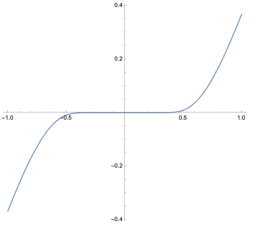
x is 3-critical for f if f'(x) = 0 and either (i) f''(x) = f'''(x) = 0 or (ii) f''(x) > 0.
From the definition of p-criticality through neighborhoods, it is immediate that if x is a local minimum of f \colon \reals \to \reals, then x is p-criticality for all p \geq 1. It turns out the converse is NOT true in general.
However, if we additionally know that f is real-analytic, then the converse is true. The following propsition is an easy consequence of our characterization of 1D p-criticality through derivatives.
p-criticality for arbitrary dimension
Now let us move on to arbitrary dimension d. We may consider the following definitions for x being p-critical for f. We shall see that, in general, none of these definitions are equivalent.
Some observations:
Definitions (a), (b) and (c) are equivalent for p=1, 2, 3. See the next section for a proof for the case p=3 (the cases p=1,2 are left as an exercise).
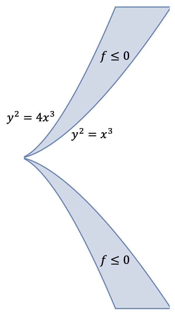
Surprisingly, for p \geq 4, these definitions are not equivalent, and in fact (c) implies (b) implies (a). However, the converses are not true even for polynomial functions. In the “Counterexamples” section below, we give counterexamples to this effect.
From the definition through neighbhorhoods and the implications (c) implies (b) implies (a), it is immediate that if x is a local minimum of f, then x is p-critical for all p (for all three definitions). We already saw that the converse is not true in general, even for d=1. What if we restrict f to be real-analytic or even polynomial? For an answer, see the penultimate section of this blog.
Based on the equivalent 1D definitions of p-criticality, we might also suggest a fourth definition for arbitrary dimension d:
- [through series] x is p-critical through series if f_p has a local minimum at x.
However, this is an unsatisfying definition because it is NOT true that if x is a local minimum then x is p-critical through series, as the next counterexample indicates.
Third-order critical points (p=3)
Let’s show that that definitions (a), (b), (c) are equivalent when p=3. This is not true for p \geq 4 — see the subsequent section.
This result about 3-criticality is well-known — see for example Section 3 in this paper of Anandkumar and Ge. In a similar spirit, Ahmadi and Zhang give a closely related characterization of local minima of cubic polynomials, e.g., see slide 9 here.
Counterexamples
What is the “right” definition of p-criticality?
In the previous two counterexamples, we saw that there exists polynomial f such that 0 is p-critical through curves for all p \geq 1 for f, and yet 0 is not a local minimum of f. Do such examples exist for p-criticality through neighborhoods? It turns out the answer is no!
For a proof of this proposition, you will have to wait for the next blog post! Note that in general p(k, d) > k, as exhibited by counterexample (3) — contrast this with the 1D case where p(k, 1) = k.
So among the three definitions of p-criticality (through straight lines, curves, neighborhoods), which one the deserves the title of p-criticality (no “through …” qualifier)? Given Proposition 2 and the polynomial counterexamples, I argue that it is p-criticality through neighborhoods (and indeed this seems to be somewhat reflected in the literature). However, since p-criticality through neighborhoods is the strongest definition, it may be hard to find such points.
On the complexity of finding p-critical points
Anandkumar and Ge show that it is possible to efficiently find points which are 3-critical through neighborhoods. In a related line of work, Ahmadi and Zhang investigate the complexity of finding local minima for polynomials (especially for cubic polynomials): see these slides and this paper.
On the other hand, Anandkumar and Ge show that even finding points which are 4-critical through neighborhoods is NP-hard. This shows that optimization algorithms often have a hard time avoiding higher-order (aka flat) critical points. Therefore, often one tries to show a function under consideration does not have higher-order critical points: this leads us to the notion of Morse/Morse-Bott/Morse-Kirwan functions. Much can be said about these (and they are very useful) — perhaps the subject of future blog posts!
How to cite
If you would like to cite this post, you can use:
@misc{criscitiello2024higherordercriticalpoints,
  author       = {Christopher Criscitiello},
  title        = {Higher-order critical points: definitions and curiosities},
  year         = {2024},
  month        = sep,
  howpublished = {\url{https://ccriscitiello.github.io/downhillblog/posts/higher_order_critical_points/}},
  note         = {Blog post, published September 20, 2024; updated October 3, 2024}
}Acknowledgments: We thank Nicolas Boumal for several helpful suggestions and improvements.