Gradient flows and the Łojasiewicz inequality, with an application to higher-order criticality

We show that every saddle point of a real-analytic function has a gradient flow line converging to it. We use this fact to prove a claim made in our previous blog post on higher-order criticality: if x is a p-critical point of a real-analytic function f for all positive integers p, then x is a local minimum of f. The key tools used throughout are gradient flows and the Łojasiewicz inequality.

\newcommand{\abs}[1]{\left|{#1}\right|} \newcommand{\argmax}[1]{\underset{#1}{\operatorname{argmax}}} \newcommand{\argmin}[1]{\underset{#1}{\operatorname{argmin}}} \newcommand{\bareta}{{\overline{\eta}}} \newcommand{\barf}{{\overline{f}}} \newcommand{\barg}{{\overline{g}}} \newcommand{\barM}{\overline{\mathcal{M}}} \newcommand{\barnabla}{\overline{\nabla}} \newcommand{\barRcurv}{\bar{\mathcal{R}}} \newcommand{\barRmop}{\bar{R}_\mathrm{m}} \newcommand{\barRmoptensor}{\mathbf{{\bar{R}_\mathrm{m}}}} \newcommand{\barx}{{\overline{x}}} \newcommand{\barX}{{\overline{X}}} \newcommand{\barxi}{{\overline{\xi}}} \newcommand{\bary}{{\overline{y}}} \newcommand{\barY}{{\overline{Y}}} \newcommand{\bfeta}{{\bm{\eta}}} \newcommand{\bfF}{\mathbf{F}} \newcommand{\bfOmega}{\boldsymbol{\Omega}} \newcommand{\bfR}{\mathbf{R}} \newcommand{\bftheta}{{\bm{\theta}}} \newcommand{\bfX}{{\mathbf{X}}} \newcommand{\bfxi}{{\bm{\xi}}} \newcommand{\bfY}{{\mathbf{Y}}} \newcommand{\calA}{\mathcal{A}} \newcommand{\calB}{\mathcal{B}} \newcommand{\calP}{\mathcal{P}} \newcommand{\calC}{\mathcal{C}} \newcommand{\calE}{\mathcal{E}} \newcommand{\calF}{\mathcal{F}} \newcommand{\calG}{\mathcal{G}} \newcommand{\calH}{\mathcal{H}} \newcommand{\calJ}{\mathcal{J}} \newcommand{\calK}{\mathcal{K}} \newcommand{\calL}{\mathcal{L}} \newcommand{\ones}{\textbf{1}} \newcommand{\calM}{\mathcal{M}} \newcommand{\calN}{\mathcal{N}} \newcommand{\calO}{\mathcal{O}} \newcommand{\calS}{\mathcal{S}} \newcommand{\calT}{\mathcal{T}} \newcommand{\calU}{\mathcal{U}} \newcommand{\calV}{\mathcal{V}} \newcommand{\calW}{\mathcal{W}} \newcommand{\calX}{\mathcal{X}} \newcommand{\Cm}{{\mathbb{C}^m}} \newcommand{\CN}{{\mathbb{C}^{\,N}}} \newcommand{\Cn}{\mathbb{C}^n} \newcommand{\CNN}{{\mathbb{C}^{\ N\times N}}} \newcommand{\Cnn}{\mathbb{C}^{n\times n}} \newcommand{\CnotR}{{\mathbb{C}\ \backslash\mathbb{R}}} \newcommand{\col}{\operatorname{col}} \newcommand{\im}{\operatorname{im}} \newcommand{\complex}{{\mathbb{C}}} \newcommand{\Cov}{\mathbf{C}} \newcommand{\Covm}{C} \newcommand{\Ric}{\mathrm{Ric}} \newcommand{\Rmcurv}{\mathrm{Rm}} \newcommand{\D}{\mathrm{D}} \newcommand{\dblquote}[1]{``#1''} \newcommand{\dd}[1]{\frac{\mathrm{d}}{\mathrm{d}#1}} \newcommand{\ddiag}{\mathrm{ddiag}} \newcommand{\ddp}[2]{\frac{\partial #1}{\partial #2}} \newcommand{\Ddq}{\frac{\D}{\dq}} \newcommand{\dds}{\frac{\mathrm{d}}{\mathrm{d}s}} \newcommand{\Ddt}{\frac{\D}{\dt}} \newcommand{\ddt}{\frac{\mathrm{d}}{\mathrm{d}t}} \newcommand{\Ddttwo}{\frac{\D^2}{\dt^2}} \newcommand{\defeq}{\triangleq} \newcommand{\Dexp}{\D\!\exp} \newcommand{\error}{\mathrm{error}} \newcommand{\diag}{\mathrm{diag}} \newcommand{\Diag}{\mathrm{Diag}} \newcommand{\Vol}{\mathrm{Vol}} \newcommand{\polylog}{\mathrm{polylog}} \newcommand{\poly}{\mathrm{poly}} \newcommand{\dist}{\mathrm{dist}} \newcommand{\Dlog}{\D\!\log} \newcommand{\dmu}{\mathrm{d}\mu} \newcommand{\dphi}{\mathrm{d}\phi} \newcommand{\dq}{\mathrm{d}q} \newcommand{\ds}{\mathrm{d}s} \newcommand{\dt}{\mathrm{d}t} \newcommand{\dtau}{\mathrm{d}\tau} \newcommand{\dtheta}{\mathrm{d}\theta} \newcommand{\du}{\mathrm{d}u} \newcommand{\dx}{\mathrm{d}x} \newcommand{\Ebad}{E_\textrm{bad}} \newcommand{\Egood}{E_\textrm{good}} \newcommand{\eig}{{\mathrm{eig}}} \newcommand{\ellth}{$\ell$th } \newcommand{\embdist}{\mathrm{embdist}} \newcommand{\ER}{{Erd\H{o}s-R\'enyi }} \newcommand{\Exp}{\mathrm{Exp}} \newcommand{\expect}{\mathbb{E}} \newcommand{\expectt}[1]{\mathbb{E}\left\{{#1}\right\}} \newcommand{\expp}[1]{{\exp\!\big({#1}\big)}} \newcommand{\feq}{{f_\mathrm{eq}}} \newcommand{\FIM}{\mathbf{F}} \newcommand{\FIMm}{F} \newcommand{\floor}[1]{\lfloor #1 \rfloor} \newcommand{\flow}{f_{\mathrm{low}}} \newcommand{\FM}{\mathfrak{F}(\M)} \newcommand{\frobnorm}[2][F]{\left\|{#2}\right\|_\mathrm{#1}} \newcommand{\frobnormbig}[1]{\big\|{#1}\big\|_\mathrm{F}} \newcommand{\frobnormsmall}[1]{\|{#1}\|_\mathrm{F}} \newcommand{\GLr}{{\mathbb{R}^{r\times r}_*}} \newcommand{\Gr}{\mathrm{Gr}} \newcommand{\grad}{\mathrm{grad}} \newcommand{\Hess}{\mathrm{Hess}} \newcommand{\HH}{\mathrm{H}} \newcommand{\Id}{\operatorname{Id}} % need to be distinguishable from identity matrix \newcommand{\II}{I\!I} \newcommand{\inj}{\mathrm{inj}} \newcommand{\inner}[2]{\left\langle{#1},{#2}\right\rangle} \newcommand{\innerbig}[2]{\big\langle{#1},{#2}\big\rangle} \newcommand{\innersmall}[2]{\langle{#1},{#2}\rangle} \newcommand{\ith}{$i$th } \newcommand{\jth}{$j$th } \newcommand{\Klow}{{K_{\mathrm{low}}}} \newcommand{\Kmax}{K_{\mathrm{max}}} \newcommand{\kth}{$k$th } \newcommand{\Kup}{{K_{\mathrm{up}}}} \newcommand{\Klo}{{K_{\mathrm{lo}}}} \newcommand{\lambdamax}{\lambda_\mathrm{max}} \newcommand{\lambdamin}{\lambda_\mathrm{min}} \newcommand{\langevin}{\mathrm{Lang}} \newcommand{\langout}{\mathrm{LangUni}} \newcommand{\length}{\operatorname{length}} \newcommand{\Log}{\mathrm{Log}} \newcommand{\longg}{{\mathrm{long}}} \newcommand{\M}{\mathcal{M}} \newcommand{\mle}{{\mathrm{MLE}}} \newcommand{\mlez}{{\mathrm{MLE0}}} \newcommand{\MSE}{\mathrm{MSE}} \newcommand{\N}{\mathrm{N}} \newcommand{\norm}[1]{\left\|{#1}\right\|} \newcommand{\nulll}{\operatorname{null}} \newcommand{\hull}{\mathrm{hull}} \newcommand{\Od}{{\mathrm{O}(d)}} \newcommand{\On}{{\mathrm{O}(n)}} \newcommand{\One}{\mathds{1}} \newcommand{\Op}{{\mathrm{O}(p)}} \newcommand{\opnormsmall}[1]{\|{#1}\|_\mathrm{op}} \newcommand{\p}{\mathcal{P}} \newcommand{\pa}[1]{\left(#1\right)} \newcommand{\paa}[1]{\left\{#1\right\}} \newcommand{\pac}[1]{\left[#1\right]} \newcommand{\pdd}[1]{\frac{\partial}{\partial #1}} \newcommand{\polar}{\mathrm{polar}} \newcommand{\Precon}{\mathrm{Precon}} \newcommand{\proj}{\mathrm{proj}} \newcommand{\Proj}{\mathrm{Proj}} \newcommand{\ProjH}{\mathrm{Proj}^h} \newcommand{\PSD}{\mathrm{PSD}} \newcommand{\ProjV}{\mathrm{Proj}^v} \newcommand{\qf}{\mathrm{qf}} \newcommand{\rank}{\operatorname{rank}} \newcommand{\Rball}{R_{\mathrm{ball}}} \newcommand{\Rcurv}{\mathcal{R}} \newcommand{\Rd}{{\mathbb{R}^{d}}} \newcommand{\Rdd}{{\mathbb{R}^{d\times d}}} \newcommand{\Rdp}{{\mathbb{R}^{d\times p}}} \newcommand{\reals}{{\mathbb{R}}} \newcommand{\Retr}{\mathrm{R}} \newcommand{\Rk}{{\mathbb{R}^{k}}} \newcommand{\Rm}{{\mathbb{R}^m}} \newcommand{\Rmle}{{\hat\bfR_\mle}} \newcommand{\Rmm}{{\mathbb{R}^{m\times m}}} \newcommand{\Rmn}{{\mathbb{R}^{m\times n}}} \newcommand{\Rmnr}{{\mathbb{R}_r^{m\times n}}} \newcommand{\Rmop}{R_\mathrm{m}} \newcommand{\Rmoptensor}{\mathbf{{R_\mathrm{m}}}} \newcommand{\Rmr}{\mathbb{R}^{m\times r}} \newcommand{\RMSE}{\mathrm{RMSE}} \newcommand{\Rn}{{\mathbb{R}^n}} \newcommand{\Rnk}{\mathbb{R}^{n\times k}} \newcommand{\Rnm}{\mathbb{R}^{n\times m}} \newcommand{\Rnn}{{\mathbb{R}^{n\times n}}} \newcommand{\RNN}{{\mathbb{R}^{N\times N}}} \newcommand{\Rnp}{{\mathbb{R}^{n\times p}}} \newcommand{\Rnr}{\mathbb{R}^{n\times r}} \newcommand{\Rp}{{\mathbb{R}^{p}}} \newcommand{\Rpp}{\mathbb{R}^{p\times p}} \newcommand{\Rrn}{{\mathbb{R}^{r\times n}}} \newcommand{\Rrr}{\mathbb{R}^{r\times r}} \newcommand{\Rtt}{{\mathbb{R}^{3\times 3}}} \newcommand{\sbd}[1]{\sbdop\!\left({#1}\right)} \newcommand{\sbdop}{\operatorname{symblockdiag}} \newcommand{\sbdsmall}[1]{\sbdop({#1})} \newcommand{\Sd}{\mathbb{S}^{d}} \newcommand{\Sdd}{{\mathbb{S}^{d\times d}}} \newcommand{\short}{{\mathrm{short}}} \newcommand{\sigmamax}{\sigma_{\operatorname{max}}} \newcommand{\sigmamin}{\sigma_{\operatorname{min}}} \newcommand{\sign}{\mathrm{sign}} \newcommand{\ske}{\operatorname{skew}} \newcommand{\Skew}{\operatorname{Skew}} \newcommand{\skeww}[1]{\operatorname{skew}\!\left( #1 \right)} \newcommand{\Sm}{\mathbb{S}^{m-1}} \newcommand{\smallfrobnorm}[1]{\|{#1}\|_\mathrm{F}} \newcommand{\Smdmd}{{\mathbb{S}^{md\times md}}} \newcommand{\Smm}{{\mathbb{S}^{m\times m}}} \newcommand{\Sn}{\mathbb{S}^{n-1}} \newcommand{\Snn}{{\mathbb{S}^{n\times n}}} \newcommand{\So}{{\mathbb{S}^{1}}} \newcommand{\SOd}{\operatorname{SO}(d)} \newcommand{\SOdm}{\operatorname{SO}(d)^m} \newcommand{\son}{{\mathfrak{so}(n)}} \newcommand{\SOn}{{\mathrm{SO}(n)}} \newcommand{\sot}{{\mathfrak{so}(3)}} \newcommand{\SOt}{{\mathrm{SO}(3)}} \newcommand{\sotwo}{{\mathfrak{so}(2)}} \newcommand{\SOtwo}{{\mathrm{SO}(2)}} \newcommand{\Sp}{{\mathbb{S}^{2}}} \newcommand{\spann}{\mathrm{span}} \newcommand{\gspan}{\mathrm{gspan}} \newcommand{\Spp}{{\mathbb{S}^{p\times p}}} \newcommand{\sqfrobnorm}[2][F]{\frobnorm[#1]{#2}^2} \newcommand{\sqfrobnormbig}[1]{\frobnormbig{#1}^2} \newcommand{\sqfrobnormsmall}[1]{\frobnormsmall{#1}^2} \newcommand{\sqnorm}[1]{\left\|{#1}\right\|^2} \newcommand{\Srr}{{\mathbb{S}^{r\times r}}} \newcommand{\St}{\mathrm{St}} \newcommand{\Cent}{\mathrm{Centered}} \newcommand{\Holl}{\mathrm{Hollow}} \newcommand{\Stdpm}{\St(d, p)^m} \newcommand{\Stnp}{{\mathrm{St}(n,p)}} \newcommand{\Stwo}{{\mathbb{S}^{2}}} \newcommand{\symm}[1]{\symmop\!\left( #1 \right)} \newcommand{\symmop}{\operatorname{sym}} \newcommand{\symmsmall}[1]{\symmop( #1 )} \newcommand{\Symn}{\mathrm{Sym}(n)} \newcommand{\Symnminp}{\mathrm{Sym}(n-p)} \newcommand{\Symp}{\mathrm{Sym}(p)} \newcommand{\Sym}{\mathrm{Sym}} \newcommand{\T}{\mathrm{T}} \newcommand{\TODO}[1]{{\color{red}{[#1]}}} \newcommand{\trace}{\mathrm{Tr}} \newcommand{\Trace}{\mathrm{Tr}} \newcommand{\Trans}{\mathrm{Transport}} \newcommand{\Transbis}[2]{\mathrm{Transport}_{{#1}}({#2})} \newcommand{\transpose}{^\top\! } \newcommand{\uniform}{\mathrm{Uni}} \newcommand{\var}{\mathrm{var}} \newcommand{\vecc}{\mathrm{vec}} \newcommand{\veccc}[1]{\vecc\left({#1}\right)} \newcommand{\VV}{\mathrm{V}} \newcommand{\XM}{\mathfrak{X}(\M)} \newcommand{\xorigin}{x_{\mathrm{ref}}} \newcommand{\Zeq}{{Z_\mathrm{eq}}} \newcommand{\aref}[1]{\hyperref[#1]{A\ref{#1}}} \newcommand{\frobnorm}[1]{\left\|{#1}\right\|_\mathrm{F}} \newcommand{\sqfrobnorm}[1]{\frobnorm{#1}^2}

Introduction

In our previous blog post, we considered several definitions of p-criticality (through straight lines, curves and neighborhoods), and showed none of these definitions are equivalent. Let’s recall them here:

Definitions of p-critical point

The point x \in \reals^d is p-critical for f through “straight lines”, “curves”, or “neighborhoods” if:

1. [through straight lines] For all v \in \mathbb{R}^d, the 1D function t \mapsto f(x + t v) has a p-th order critical point at t=0.

2. [through curves] For all C^p curves \gamma with \gamma(0) = x and \gamma'(0) \neq 0, the 1D function t \mapsto f(\gamma(t)) has a p-th order critical point at t=0.

3. [through neighborhoods] There is an \epsilon > 0 and C > 0 such that f(x + v) \geq f(x) - C \|v\|^{p+1} for all v \in \reals^d such that \|v\| \leq \epsilon. (This is definition 1 in this paper of Anandkumar and Ge.)

We concluded that the “right” definition of p-criticality is through neighborhoods, due to the following two properties (not enjoyed by the other definitions).

Proposition 1

If f \colon \reals^d \to \reals is real-analytic and 0 is p-critical through neighborhoods for all p \geq 1, then 0 is a local minimum of f.

Proposition 2

For each d \geq 1 and k \geq 1, there is a (finite) positive integer p(k,d) such that: if f \colon \reals^d \to \reals is a degree-k polynomial and 0 is p(k,d)-critical through neighborhoods, then 0 is a local minimum of f.

Counterexamples: Propositions 1 and 2

For Proposition 1, the real-analytic assumption is necessary, i.e., f being C^\infty is not enough — recall the 1D counterexample f(x) = x e^{-1/x^2} from our previous blog post.

For Proposition 2, it is easy to show that p(k, 1) = k works. However, for d > 1, p(k, d) = k is not enough — recall the counterexample f(x,y) = y^2 - x^2 y - x y^2 from our previous blog post. We argued that (0,0) is 3-critical for f, but it is not a local minimum (hence p(3, 2) > 3). Exercise: Show that p(3, 2) = 5 works.

Propositions 1 and 2 are consequences of the following result.

Proposition 3

Let f \colon \reals^d \to \reals be real-analytic, with f(0) = 0, \nabla f(0) = 0. If 0 is not a local minimum of f, then there exists x_0 \in \reals^d \setminus \{0\} such that positive gradient flow (+gradflow) started from x_0 converges to 0.

Proposition 3 is probably known — see these papers of Moussu, Nowel and Szafraniec, and Szafraniec. We present a proof at the end of this post. This proof may be new, and, more importantly, it is self-contained and hopefully easy to parse!

The key tools to prove Propositions 1, 2, 3 are gradient flows and the Łojasiewicz inequality.

Counterexample: Proposition 3

The assumption that f is real-analytic in Propostion 3 is necessary, i.e., it is not enough for f to be only C^\infty. Indeed, consider a smooth 1D function which oscillates infinitely often, like the following: f(x) = \sin(6\pi/x) e^{-1/x^2}. Non-constant gradient flow trajectories cannot converge to the origin because there are 1-critical points arbitrarily close to it (on both sides).

The function above is somewhat pathological as its set of 1-critical points is not a smooth manifold. What if we additionally assume the set of 1-critical points of f is a smooth manifold? Even this is not enough for Proposition 3 to hold: an example is furnished by the so-called “Mexican hat function” and variants thereof (see pages 4-5 in this paper by Absil, Mahony and Andrews).

Figure 1: Plot of f(x) = \sin(6\pi/x) e^{-1/x^2}.

Gradient flows

Let f \colon \reals^d \to \reals be C^\infty. A positive gradient flow trajectory started at x_0 \in \reals^d is a solution of the ODE \begin{align}\tag{$+$gradflow} x'(t) = \nabla f(x(t)), \quad \quad t \in \reals, \quad \quad x(0) = x_0. \end{align} Likewise, negative gradient flow is a solution of \begin{align}\tag{$-$gradflow} x'(t) = -\nabla f(x(t)), \quad \quad t \in \reals, \quad \quad x(0) = x_0. \end{align} A gradient flow is always defined on some open interval around t = 0; however, it may not be defined on all of \reals. If \nabla f(x_0) is nonzero then gradient flow never reaches a 1-critical point in finite time (since the flow map \Phi defined below is a diffeomorphism in an appropriate sense). Therefore, the quantity f(x(t)) is always increasing for positive gradient flow with \nabla f(x_0) \neq 0. This is because \frac{d}{dt}[f(x(t))] = \mathrm{D} f(x(t))[x'(t)] = \|\nabla f(x(t))\|^2 > 0 \quad \quad \text{for all $t$}. (And likewise the function value decreases for negative gradient flow.)

We define the positive gradient flow map \Phi by \begin{align}\tag{flowmap} \Phi(x_0, t) = x(t) \end{align} where x(\cdot) is the positive gradient flow starting at x_0. The flow map \Phi is defined on a (open) subset of \reals^d \times \reals (this domain is called the flow’s maximal flow domain). It is a fact that \Phi is differentiable on its domain. Further, for a given t, the map x \mapsto \Phi(x, t) is a diffeomorphism (from the set of points on which it is well defined and onto its image). For more information on vector-field flows more generally, we recommend Chapter 9 “Integral Curves and Flows” of Introduction to Smooth Manifolds by John Lee.

For any F \in \reals, let \tau(F, x_0) denote the first time t \geq 0 at which the positive gradient flow (+gradflow) leaves the sublevel set \{x \in \reals^d : f(x) < F\}, with the convention that \tau(F, x_0) = +\infty if the flow never leaves the sublevel set in finite time. As a shorthand, we also define \tau(x) := \tau(0, x). Note that if \nabla f(x_0) \neq 0 and \tau(F, x_0) is finite, then it is the only time t for which f(x(t)) = F, since f(x(t)) is increasing. For a given F, we can define a map x \mapsto \tau(F, x) from \reals^d to [0, \infty]. We have the following useful fact.

Lemma 1

Let f \colon \reals^d \to \reals be C^\infty, and let x_0 \in \reals^d, F \in \reals. Assume \tau(F, x_0) is finite. Then the map x \mapsto \tau(F, x) is finite and differentiable in a neighborhood of x_0.

Proof of Lemma 1

The main idea is to apply the implicit function theorem. At the end, we also sketch another approach based on rescaling/reparameterizing the gradient flow.

We know that (x, t) = (x_0, \tau(F, x_0)) is a solution of the equation f(\Phi(x, t)) = F recalling the definition (flowmap) of the flow map \Phi. To apply the implicit function theorem, we need to check that the t-differential of f(\Phi(x, t)) is nonzero at (x, t) = (x_0, \tau(F, x_0)). Indeed, \frac{d}{dt}[f(\Phi(x_0, t))]_{t = \tau(F, x_0)} = \mathrm{D} f(\Phi(x_0, \tau(F, x_0)))[x'(\tau(F, x_0))] = \|\nabla f(x(\tau(F, x_0)))\|^2, which is nonzero since gradient flow cannot reach a 1-critical point in finite time.

Hence applying the implicit function theorem, there is a neighborhood U of x_0 and a unique differentiable function T \colon U \to \reals such that f(\Phi(x, T(x))) = F, \quad \quad \forall x \in U. Due to the uniqueness of \tau mentioned previously, we conclude that \tau(F, x) = T(x), which proves the lemma.

---

For those curious, let’s sketch an alternative approach, employing a useful trick. Consider the rescaled positive gradient flow: x’(s) = \frac{\nabla f(x(s))}{\|\nabla f(x(s)\|^2}, \quad x(0) = x_0. Recall that multiplying the vector field of a flow by a positive function just amounts to reparameterizing time, so the flow lines of x(\cdot) do not change, just their time parameterization does.

This rescaled/reparameterized flow has the property that it crosses level sets at constant speed, as \frac{d}{ds}[f(x(s))] = 1. In particular, the time s at which the flow leaves the sublevel set \{x \in \reals^d : f(x) < F\} equals s = F - f(x_0), provided F \geq f(x_0) and we are careful to control where \nabla f vanishes. We can then conclude that x \mapsto \tau(F, x) is a differentiable function of s = F - f(x), which itself is smooth.

The Łojasiewicz inequality

In the 1960s, Stanisław Łojasiewicz proved the following theorem, which is an extremely useful tool for controlling gradient flows. (Notation: throughout, B(0, \delta) denotes the open ball of radius \delta centered at the origin.)

Theorem: Łojasiewicz Inequality

Let f \colon \reals^d \to \reals be real-analytic, with f(0) = 0. There exist \delta_L > 0, c > 0, \mu \in [0, 1), such that \begin{align}\tag{Ł} \|\nabla f(x)\| \geq c |f(x)|^{\mu} \quad \quad \forall x \in B(0, \delta_L) =: U_L. \end{align}

Inequality (Ł) is known as the Łojasiewicz inequality — its proof is beyond the scope of this blog.

If f satisfies the Łojasiewicz inequality, then its gradient flows cannot stray too far from their starting points.

Lemma 2: Łojasiewicz inequality implies growth

Assume f is C^\infty, has f(0) = 0, \nabla f(0) = 0, and satisfies the Łojasiewicz inequality (Ł) with constants c, \mu in neighborhood U_L = B(0, \delta_L). There is a neighborhood U_M = B(0, \delta_M), \delta_M \leq \delta_L/2, such that if x(t) is the positive gradient flow (+gradflow) started from x_0 \in U_M with f(x_0) < 0, then x(t) \in U_L \quad \quad \text{for all $t \in [0, \tau(x_0)]$} and moreover \begin{align} \tag{localization} \|x_0 - x(t)\| \leq (c(1-\mu))^{-1} |f(x_0)|^{1-\mu} \quad \quad \text{for all $t \in [0, \tau(x_0)]$}. \end{align}

In Lemma 2, \tau(x(0)) may be either finite or infinite. If it is infinite, then x(t) must converge to a critical point of f (e.g., see the exercise at the end of this section), and x(\tau(x(0))) is that limiting point. Either way, x(\tau(x(0))) lies on the level set \{x : f(x) = 0\}.

The proof of Lemma 2 is classical and originally due to Łojasiewicz. We present a proof based on Theorem 2.2 of this paper by Absil, Mahony and Andrews.

Proof of Lemma 2

Take any x(0) \in U_L, and let T be the first time the positive gradient flow starting at x(0) leaves the set \{x \in U_L : f(x) < 0\}. For t \in [0, T), we have f(x(t)) < 0 and \begin{align*} \frac{d}{dt}\Big[ (- f (x(t)))^{1-\mu} \Big] &= (1-\mu) (- f(x(t)))^{-\mu} \frac{d}{dt}[- f(x(t))] \\ &= -(1-\mu) |f(x(t))|^{-\mu} \mathrm{D} f(x(t))[x'(t)] \\ &= -(1-\mu) |f(x(t))|^{-\mu} \|\nabla f(x(t))\| \cdot \|x'(t)\| \\ &\leq -c(1-\mu) |f(x(t))|^{-\mu} |f(x(t))|^{\mu} \cdot \|x'(t)\| \\ &= -c(1-\mu) \|x'(t)\|. \end{align*} Therefore, for any t \in [0, T) we have \begin{align*}\tag{1} \|x(0) - x(t)\| &\leq \int_0^t \|x'(\tau)\| d \tau \leq (c(1-\mu))^{-1} \Big[|f(x(0))|^{1-\mu} - |f(x(t))|^{1-\mu}\Big] \\ &\leq (c(1-\mu))^{-1} |f(x(0))|^{1-\mu}. \end{align*} The first inequality is because \int_0^t \|x'(\tau)\| d \tau is the length of the curve x(\cdot) between x(0) and x(t).

By smoothness of f and f(0) = 0, there exists a \delta_M > 0 such that \begin{align}\tag{2} \|x\| + (c(1-\mu))^{-1} |f(x)|^{1-\mu} \leq \delta_L / 2, \quad \quad \forall x \in B(0, \delta_M). \end{align}

We claim that any positive gradient flow started at x(0) \in U_M stays in B(0, \delta_L/2) \subseteq U_L until time t = \tau(x(0)). For contradiction, assume not. Then for t close to T, x(t) is arbitrarily close to the boundary of U_L (i.e., \|x(t)\| is close to \delta_L). On the other hand, inequalities (1) and (2) imply \begin{align*} \|x(t)\| \leq \|x(0)\| + (c(1-\mu))^{-1} |f(x(0))|^{1-\mu} \leq \delta_L/2 \quad \quad \forall t \in [0, T) \end{align*} which is a contradiction, proving our claim.

We conclude that x(t) \in B(0, \delta_L/2) and equation (1) holds if x(0) \in U_M and t \in [0, \tau(x(0))). We leave it as a (simple) exercise to verify this also holds for t \in [0, \tau(x(0))].

Exercise: Assume f satisfies the Łojasiewicz inequality (Ł) with constants c, \mu in U_L = B(0, \delta_L). Also assume that the gradient flow line x(\cdot) started at x(0) \in U_L stays in U_L for all t \geq 0. Show that x(t) must converge to a critical point of f. [Hint: Use Lemma 2, with a compactness argument.]

Proofs of Propositions 1 and 2: When does p-critical imply local minimum?

We are now ready to prove Proposition 4 below. Propositions 1 and 2 are immediate consequences.

Proposition 4

Suppose f \colon \reals^d \to \reals is C^\infty with f(0) = 0, and satisfies the Łojasiewicz inequality (Ł) with constants c, \mu in neighborhood U_L. If 0 is p-critical through neighborhoods for some p > (1-\mu)^{-1} - 1, then 0 is a local minimum of f.

Proof of Proposition 4

By definition of p-criticality through neighborhoods, there is a \delta_p > 0, C_p > 0 such that \begin{align}\tag{$p$-criticality} f(x) - f(0) = f(x) \geq -C_p \|x\|^{p+1} \quad \quad \forall x \in B(0, \delta_p). \end{align} Suppose, for contradiction, that 0 is not a local minimum. Then by Proposition 3 there exists a x_0 \in U_L \cap B(0, \delta_p) such that positive gradient flow x(t) started from x(0) = x_0 converges to 0 (and stays in U_L \cap B(0, \delta_p) and has f(x(t)) < 0). In particular, invoking Lemma 2, we have \|x(t)\| \leq (c(1-\mu))^{-1} |f(x(t))|^{1-\mu} \quad \quad \forall t \geq 0. On the other hand, (p-criticality) says |f(x(t)| \leq C_p \|x(t)\|^{p+1}. Putting these together, we have for all t \geq 0: \|x(t)\| \leq (c(1-\mu))^{-1} C_p^{1-\mu} \|x(t)\|^{(p+1)(1-\mu)}. This is a contradiction since (p+1)(1-\mu) > 1 and \|x(t)\| \to 0.

Proposition 1 follows immediately from Proposition 4 and Łojasiewicz’s theorem previously stated.

Proposition 2 follows immediately from Proposition 4, and bounds on the best Łojasiewicz exponent \mu given by D’Acunto and Kurdyka. Specifically, D’Acunto and Kurdyka show that if f \colon \reals^d \to \reals is a degree-k polynomial, then f satisfies the Łojasiewicz inequality with exponenent \mu = 1 - (3 k)^{-d}.

Proof of Proposition 3: every saddle has a gradient flow line converging to it

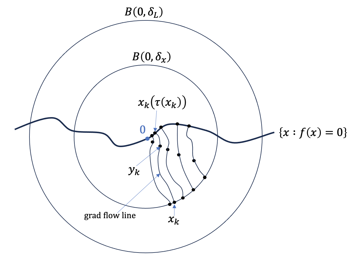
It remains to only prove Proposition 3. The idea is simple. Choose a sequence of points y_0, y_1, \ldots converging to 0 with f(y_k) < 0. For each y_k we look at the positive gradient flow line y_k(\cdot) starting at y_k until it leaves the sublevel set \{x : f(x) < 0\}. By Lemma 2, the endpoints y_k(\tau(y_k)) of the flow lines also converge to 0.

Now run the negative gradient flow starting from y_k until it first hits the boundary of B(0, \delta_x), \delta_x > 0; call the intersection point x_k. Then we know that the positive gradient flow line starting at x_k ends at y_k(\tau(y_k)), which converges to 0 as k \to \infty.

The sequence x_0, x_1, \ldots accumulates to some x_\infty on the boundary of B(0, \delta_x). It stands to reason that the positive gradient flow line started from x_\infty converges to 0. This is indeed true. Let’s look at the details.

Figure 2: Diagram corresponding to proof of Proposition 3.

Proof of Proposition 3

We know that f satisfyies the Łojasiewicz inequality (Ł) with constants c, \mu in a neighborhood U_L = B(0, \delta_L). By Lemma 2, we know there is a neighborhood U_M = B(0, \delta_M), \delta_M \leq \delta_L/2, such that if x(0) \in U_M and f(x(0)) < 0 then x(t) \in U_L for all t \in [0, \tau(x(0))].

Constructing the sequence \mathbf{y_0, y_1, \ldots \to 0}: Since 0 is not a local minimum, there is a sequence of points y_0, y_1, \ldots in U_M which converges to 0, and satisfies f(y_k) < 0 for all k. Let y_k(t) denote positive gradient flow started at y_k(0) = y_k. Equation (localization) of Lemma 2, tells us that the entire trajectories \{y_k(t) : t \in [0, \tau(y_k)]\} converge to 0, since y_k \to 0 and f(y_k) \to 0. In particular, we conclude f(y_k(\tau(y_k))) = 0, and y_k(\tau(y_k)) converges to 0 as k \to \infty.

Constructing the sequence \mathbf{x_0, x_1, \ldots \to x_\infty}: Consider the negative gradient flow lines started from each y_k. Observe that each of these flows must eventually leave the ball U_L (otherwise they are trapped and must converge to a critical point, which must have function value 0 by the Łojasiewicz inequality, a contradiction). Fix \delta_x \in (\delta_M, \delta_L). For each k, let x_k be the first point where this negative gradient flow crosses the boundary of B(0, \delta_x) (so \|x_k\| = \delta_x).

Let x_k(t) denote the positive gradient flow starting from x_k(0) = x_k. Without loss of generality (by compactness and taking a convergent subsequence), we can assume x_0, x_1, x_2, \ldots converge to some x_\infty (of course with \|x_\infty\| = \delta_x). Let’s summarize what we know about the positive gradient flows x_k(t):

1. Each flow starts at x_k(0) = x_k on the boundary of B(0, \delta_x), and f(x_k) < 0.

2. x_k(t) \in U_L for all k \geq 0 and t \in [0, \tau(x(0))].

3. x_k(\tau(x_k)) = y_k(\tau(y_k)) converges to 0, and f(x_k(\tau(x_k))) = 0 for all k \geq 0.

Finishing up: To conclude, we want to show that x_\infty(t), the positive gradient flow starting from x_\infty, converges to 0 as t \to \tau(x_\infty). That is, we want to show that for each \epsilon > 0, there is a T \in (0,\tau(x_\infty)) such that \|x_\infty(t)\| \leq \epsilon for all t \in [T, \tau(x_\infty)).

So let \epsilon \in (0, \delta_x). Choose K big enough so that \|x_k(\tau(x_k))\| \leq \epsilon / 4 for all k \geq K (which we can do by property iii). Equation (localization) of Lemma 2 gives us \delta_x / 2 < \delta_x - \epsilon/4 \leq \|x_k - x_k(\tau(x_k))\| \leq (c(1-\mu))^{-1}|f(x_k)|^{1-\mu} for all k \geq K. In other words, this gives us a lower bound on |f(x_k)| in terms of \delta_x.

Define F_\epsilon < 0 through (c(1-\mu))^{-1} |F_\epsilon|^{1-\mu} = \epsilon / 4. From this and \epsilon / 4 < \delta_x / 2, we find that |F_\epsilon| < |f(x_k)| for all k \geq K, and so 0 < \tau(F_\epsilon, x_k) < \tau(x_k) for k \geq K. Additionally, equation (localization) implies \begin{align}\tag{3} \|x_k(\tau(F_\epsilon, x_k))\| \leq \|x_k(\tau(x_k))\| + (c(1-\mu))^{-1} |F_\epsilon|^{1-\mu} \leq \epsilon/4 + \epsilon/4 = \epsilon/2 \quad \quad \forall k \geq K. \end{align}

By continuity of the flow map \Phi and continuity of x \mapsto \tau(F_\epsilon, x) (by Lemma 1), we have \lim_{k \to \infty} \Phi(x_k, \tau(F_\epsilon, x_k)) = \Phi(x_\infty, \tau(F_\epsilon, x_\infty)) = x_{\infty}(\tau(F_\epsilon, x_\infty)), and \|x_{\infty}(\tau(F_\epsilon, x_\infty))\| \leq \epsilon/2 by (3). Invoking equation (localization) one more time, we conclude \|x_{\infty}(t)\| \leq \|x_{\infty}(\tau(F_\epsilon, x_\infty))\| + (c(1-\mu))^{-1} |F_\epsilon|^{1-\mu} \leq \epsilon / 2 + \epsilon / 4 \leq \epsilon for all t \in [\tau(F_\epsilon, x_\infty), \tau(x_\infty)), as desired.

How to cite

If you would like to cite this post, you can use:

@misc{criscitiello2024gradientflowslojasiewicz,
  author       = {Christopher Criscitiello and Quentin Rebjock},
  title        = {Gradient flows and the {\L}ojasiewicz inequality, with an application to higher-order criticality},
  year         = {2024},
  month        = oct,
  howpublished = {\url{https://ccriscitiello.github.io/downhillblog/posts/Loja_p_implies_local/}},
  note         = {Blog post, published October 3, 2024}
}

---

Acknowledgements: We thank Nicolas Boumal for several helpful pointers.